机器学习:用初等数学解读逻辑回归

2015-11-03 龙心尘、寒小阳

摘自:http://my.csdn.net/longxinchen_ml

为了降低理解难度,本文试图用最基础的初等数学来解读逻辑回归,少用公式,多用图形来直观解释推导公式的现实意义,希望使读者能够对逻辑回归有更直观的理解。

逻辑回归问题的通俗几何描述

逻辑回归处理的是分类问题。我们可以用通俗的几何语言重新表述它:
空间中有两群点,一群是圆点“〇”,一群是叉点“X”。我们希望从空间中选出一个分离边界,将这两群点分开。

注:分离边界的维数与空间的维数相关。如果是二维平面,分离边界就是一条线(一维)。如果是三维空间,分离边界就是一个空间中的面(二维)。如果是一维直线,分离边界就是直线上的某一点。不同维数的空间的理解下文将有专门的论述。

为了简化处理和方便表述,我们做以下4个约定:

  1. 我们先考虑在二维平面下的情况。
  2. 而且,我们假设这两类是线性可分的:即可以找到一条最佳的直线,将两类点分开。
  3. 用离散变量y表示点的类别,y只有两个可能的取值。y=1表示是叉点“X”,y=0表示是是圆点“〇”。
  4. 点的横纵坐标用表示。

于是,现在的问题就变成了:怎么依靠现有这些点的坐标和标签(y),找出分界线的方程。

如何用解析几何的知识找到逻辑回归问题的分界线?
  1. 我们用逆推法的思路:
    假设我们已经找到了这一条线,再寻找这条线的性质是什么。根据这些性质,再来反推这条线的方程。
  2. 这条线有什么性质呢?
    首先,它能把两类点分开来。——好吧,这是废话。( ̄▽ ̄)”
    然后,两类点在这条线的法向量p上的投影的值的正负号不一样,一类点的投影全是正数,另一类点的投影值全是负数

    • 首先,这个性质是非常好,可以用来区分点的不同的类别
    • 而且,我们对法向量进行规范:只考虑延长线通过原点的那个法向量p。这样的话,只要求出法向量p,就可以唯一确认这条分界线,这个分类问题就解决了。


  3. 还有什么方法能将法向量p的性质处理地更好呢?
    因为计算各个点到法向量p投影,需要先知道p的起点的位置,而起点的位置确定起来很麻烦,我们就干脆将法向量平移使其起点落在坐标系的原点,成为新向量p’。因此,所有点到p’的投影也就变化了一个常量。

    假设这个常量为,p’向量的横纵坐标为。空间中任何一个点到p’的投影就是,再加上前面的常量值就是:

看到上面的式子有没有感到很熟悉?这不就是逻辑回归函数中括号里面的部分吗?

就可以根据z的正负号来判断点x的类别了。

从概率角度理解z的含义。

由以上步骤,我们由点x的坐标得到了一个新的特征z,那么:

z的现实意义是什么呢?

首先,我们知道,z可正可负可为零。而且,z的变化范围可以一直到正负无穷大。

z如果大于0,则点x属于y=1的类别。而且z的值越大,说明它距离分界线的距离越大,更可能属于y=1类。

那可否把z理解成点x属于y=1类的概率P(y=1|x) (下文简写成P)呢?显然不够理想,因为概率的范围是0到1的。

但是我们可以将概率P稍稍改造一下:令Q=P/(1-P),期望用Q作为z的现实意义。我们发现,当P的在区间[0,1]变化时,Q在[0,+∞)区间单调递增。函数图像如下(以下图像可以直接在度娘中搜“x/(1-x)”,超快):

但是Q的变化率在[0,+∞)还不够,我们是希望能在(-∞,+∞)区间变化的。而且在P=1/2的时候刚好是0。这样才有足够的解释力。

注:因为P=1/2说明该点属于两个类别的可能性相当,也就是说这个点恰好在分界面上,那它在法向量的投影自然就是0了。

而在P=1/2时,Q=1,距离Q=0还有一段距离。那怎么通过一个函数变换然它等于0呢?有一个天然的函数log,刚好满足这个要求。
于是我们做变换R=log(Q)=log(P/(1-P)),期望用R作为z的现实意义。画出它的函数图像如图:

这个函数在区间[0,1]中可正可负可为零,单调地在(-∞,+∞)变化,而且1/2刚好就是唯一的0值!基本完美满足我们的要求。
回到我们本章最初的问题,

“我们由点x的坐标得到了一个新的特征z,那么z的具体意义是什么呢?”

由此,我们就可以将z理解成x属于y=1类的概率P经过某种变换后对应的值。也就是说,z= log(P/(1-P))。反过来就是P=。图像如下:

这两个函数log(P/(1-P)) 、看起来熟不熟悉?

这就是传说中的logit函数和sigmoid函数!

小小补充一下:

  • 在概率理论中,Q=P/(1-P)的意义叫做赔率(odds)。世界杯赌过球的同学都懂哈。赔率也叫发生比,是事件发生和不发生的概率比。
  • 而z= log(P/(1-P))的意义就是对数赔率或者对数发生比(log-odds)。

于是,我们不光得到了z的现实意义,还得到了z映射到概率P的拟合方程:

有了概率P,我们顺便就可以拿拟合方程P=来判断点x所属的分类:

当P>=1/2的时候,就判断点x属于y=1的类别;当P<1/2,就判断点x属于y=0的类别。

构造代价函数求出参数的值

到目前为止我们就有两个判断某点所属分类的办法,一个是判断z是否大于0,一个是判断g(z)是否大于1/2。
然而这并没有什么X用,

以上的分析都是基于“假设我们已经找到了这条线”的前提得到的,但是最关键的三个参数仍未找到有效的办法求出来。

还有没有其他的性质可供我们利用来求出参数的值?

  • 我们漏了一个关键的性质:这些样本点已经被标注了y=0或者y=1的类别!
  • 我们一方面可以基于z是否大于0或者g(z) 是否大于1/2来判断一个点的类别,另一方又可以依据这些点已经被标注的类别与我们预测的类别的插值来评估我们预测的好坏。
  • 这种衡量我们在某组参数下预估的结果和实际结果差距的函数,就是传说中的代价函数Cost Function。
  • 当代价函数最小的时候,相应的参数就是我们希望的最优解。

由此可见,设计一个好的代价函数,将是我们处理好分类问题的关键。而且不同的代价函数,可能会有不同的结果。因此更需要我们将代价函数设计得解释性强,有现实针对性。

为了衡量“预估结果和实际结果的差距”,我们首先要确定“预估结果”“实际结果”是什么。

  • “实际结果”好确定,就是y=0还是y=1。
  • “预估结果”有两个备选方案,经过上面的分析,我们可以采用z或者g(z)。但是显然g(z)更好,因为g(z)的意义是概率P,刚好在[0,1]范围之间,与实际结果{0,1}很相近,而z的意思是逻辑发生比,范围是整个实数域(-∞,+∞),不太好与y={0,1}进行比较。

接下来是衡量两个结果的“差距”。

  • 我们首先想到的是y-hθ(x)。
    • 但这是当y=1的时候比较好。如果y=0,则y- hθ(x)= – hθ(x)是负数,不太好比较,则采用其绝对值hθ(x)即可。综合表示如下:
    • 但这个函数有个问题:求导不太方便,进而用梯度下降法就不太方便。
    • 因为梯度下降法超出的初等数学的范围,这里就暂且略去不解释了。
  • 于是对上面的代价函数进行了简单的处理,使之便于求导。结果如下:

代价函数确定了,接下来的问题就是机械计算的工作了。常见的方法是用梯度下降法。于是,我们的平面线形可分的问题就可以说是解决了。

从几何变换的角度重新梳理我们刚才的推理过程。

回顾我们的推理过程,我们其实是在不断地将点进行几何坐标变换的过程。

  • 第一步是将分布在整个二维平面的点通过线性投影映射到一维直线中,成为点x(z)
  • 第二步是将分布在整个一维直线的点x(z)通过sigmoid函数映射到一维线段[0,1]中成为点x(g(z))。
  • 第三步是将所有这些点的坐标通过代价函数统一计算成一个值,如果这是最小值,相应的参数就是我们所需要的理想值。

对于简单的非线性可分的问题。
  1. 由以上分析可知。比较关键的是第一步,我们之所以能够这样映射是因为假设我们点集是线性可分的。但是如果分离边界是一个圆呢?考虑以下情况。
  2. 我们仍用逆推法的思路:
    • 通过观察可知,分离边界如果是一个圆比较合理。
    • 假设我们已经找到了这个圆,再寻找这个圆的性质是什么。根据这些性质,再来反推这个圆的方程
  3. 我们可以依据这个性质:
    • 圆内的点到圆心的距离小于半径,圆外的点到圆心的距离大于半径
    • 假设圆的半径为r,空间中任何一个点到原点的距离为
    • ,就可以根据z的正负号来判断点x的类别了
    • 然后令,就可以继续依靠我们之前的逻辑回归的方法来处理和解释问题了。
  4. 从几何变换的角度重新梳理我们刚才的推理过程。
    • 第一步是将分布在整个二维平面的点通过某种方式映射到一维直线中,成为点x(z)
    • 第二步是将分布在整个一维射线的点x(z)通过sigmoid函数映射到一维线段[0,1]中成为点x(g(z))。
    • 第三步是将所有这些点的坐标通过代价函数统一计算成一个值v,如果这是最小值,相应的参数就是我们所需要的理想值。


从特征处理的角度重新梳理我们刚才的分析过程

其实,做数据挖掘的过程,也可以理解成做特征处理的过程。我们典型的数据挖掘算法,也就是将一些成熟的特征处理过程给固定化的结果
对于逻辑回归所处理的分类问题,我们已有的特征是这些点的坐标,我们的目标就是判断这些点所属的分类y=0还是y=1。那么最理想的想法就是希望对坐标进行某种函数运算,得到一个(或者一些)新的特征z,基于这个特征z是否大于0来判断该样本所属的分类。

对我们上一节非线性可分问题的推理过程进行进一步抽象,我们的思路其实是:

  • 第一步,将点的坐标通过某种函数运算,得到一个新的类似逻辑发生比的特征
  • 第二步是将特征z通过sigmoid函数得到新的特征
  • 第三步是将所有这些点的特征q通过代价函数统一计算成一个值,如果这是最小值,相应的参数(r)就是我们所需要的理想值。

对于复杂的非线性可分的问题

由以上分析可知。比较关键的是第一步,如何设计转换函数。我们现在开始考虑分离边界是一个极端不规则的曲线的情况。

我们仍用逆推法的思路:

  • 通过观察等先验的知识(或者完全不观察乱猜),我们可以假设分离边界是某种6次曲线(这个曲线方程可以提前假设得非常复杂,对应着各种不同的情况)。
  • 第一步:将点的坐标通过某种函数运算,得到一个新的特征。并假设z是某种程度的逻辑发生比,通过其是否大于0来判断样本所属分类。
  • 第二步:将特征z通过sigmoid函数映射到新的特征
  • 第三步:将所有这些样本的特征q通过逻辑回归的代价函数统一计算成一个值,如果这是最小值,相应的参数就是我们所需要的理想值。相应的,分离边界其实就是方程=0,也就是逻辑发生比为0的情况嘛

多维逻辑回归的问题

以上考虑的问题都是基于在二维平面内进行分类的情况。其实,对于高维度情况的分类也类似。

高维空间的样本,其区别也只是特征坐标更多,比如四维空间的点x的坐标为。但直接运用上文特征处理的视角来分析,不过是对坐标进行参数更多的函数运算得到新的特征并假设z是某种程度的逻辑发生比,通过其是否大于0来判断样本所属分类。

而且,如果是高维线性可分的情况,则可以有更近直观的理解。

  • 如果是三维空间,分离边界就是一个空间中的一个二维平面。两类点在这个二维平面的法向量p上的投影的值的正负号不一样,一类点的投影全是正数,另一类点的投影值全是负数。
  • 如果是高维空间,分离边界就是这个空间中的一个超平面。两类点在这个超平面的法向量p上的投影的值的正负号不一样,一类点的投影全是正数,另一类点的投影值全是负数。
  • 特殊的,如果是一维直线空间,分离边界就是直线上的某一点p。一类点在点p的正方向上,另一类点在点p的负方向上。这些点在直线上的坐标可以天然理解成类似逻辑发生比的情况。可见一维直线空间的分类问题是其他所有高维空间投影到法向量后的结果,是所有逻辑回归问题的基础

多分类逻辑回归的问题

以上考虑的问题都是二分类的问题,基本就是做判断题。但是对于多分类的问题,也就是做选择题,怎么用逻辑回归处理呢?

其基本思路也是二分类,做判断题。

比如你要做一个三选一的问题,有ABC三个选项。首先找到A与BUC(”U”是并集符号)的分离边界。然后再找B与AUC的分离边界,C与AUB的分离边界。

这样就能分别得到属于A、B、C三类的概率,综合比较,就能得出概率最大的那一类了。

总结

本文的分析思路——逆推法

画图,观察数据,看出(猜出)规律,假设规律存在,用数学表达该规律,求出相应数学表达式。
该思路比较典型,是数据挖掘过程中的常见思路。

两个视角:几何变换的视角与特征处理的视角。

  1. 小结:
    • 几何变换的视角:高维空间映射到一维空间 → 一维空间映射到[0,1]区间 → [0,1]区间映射到具体的值,求最优化解
    • 特征处理的视角:特征运算函数求特征单值z → sigmoid函数求概率 → 代价函数求代价评估值,求最优化解
  2. 首先要说明的是,在逻辑回归的问题中,这两个视角是并行的,而不是包含关系。它们是同一个数学过程的两个方面
    • 比如,我们后来处理复杂的非线性可分问题的时候,看似只用的是特征处理的思路。其实,对于复杂的非线性分离边界,也可以映射到高维空间进行线性可分的处理。在SVM中,有时候某些核函数所做的映射与之非常类似。这将在我们接下来的SVM系列文章中有更加详细的说明
  3. 在具体的分析过程中,运用哪种视角都可以,各有优点
    • 比如,作者个人比较倾向几何变换的视角来理解,这方便记忆整个逻辑回归的核心过程,画几张图就够了。相应的信息都浓缩在图像里面,异常清晰。
    • 于此同时,特征处理的视角方便你思考你手上掌握的特征是什么,怎么处理这些特征。这其实的数据挖掘的核心视角。因为随着理论知识和工作经验的积累,越到后面越会发现,当我们已经拿到无偏差、倾向性的数据集,并且做过数据清洗之后,特征处理的过程是整个数据挖掘的核心过程:怎么收集这些特征,怎么识别这些特征,挑选哪些特征,舍去哪些特征,如何评估不同的特征……这些过程都是对你算法结果有决定性影响的极其精妙的精妙部分。这是一个庞大的特征工程,里面的内容非常庞大,我们将在后续的系列文章中专门讨论
    • 总的来说,几何变换视角更加直观具体,特征处理视角更加抽象宏观,在实际分析过程中,掌握着两种视角的内在关系和转换规律,综合分析,将使得你对整个数据挖掘过程有更加丰富和深刻的认识
    • 为了将这两种视角更集中地加以对比,我们专门制作了下面的图表,方便读者查阅。

原文链接:http://blog.csdn.net/longxinchen_ml/article/details/49284391

封面来源:www.taopic.com

作者介绍:

龙心尘和寒小阳:从事机器学习/数据挖掘相关应用工作,热爱机器学习/数据挖掘

『我们是一群热爱机器学习,喜欢交流分享的小伙伴,希望通过“ML学分计划”交流机器学习相关的知识,认识更多的朋友。欢迎大家加入我们的讨论群获取资源资料,交流和分享。』

联系方式:

龙心尘 johnnygong.ml@gmail.com

寒小阳 hanxiaoyang.ml@gmail.com


Essentials of Machine Learning Algorithms (with Python and R Codes)

Source: http://www.analyticsvidhya.com/blog/2015/08/common-machine-learning-algorithms/

Introduction

Google’s self-driving cars and robots get a lot of press, but the company’s real future is in machine learning, the technology that enables computers to get smarter and more personal.

– Eric Schmidt (Google Chairman)

We are probably living in the most defining period of human history. The period when computing moved from large mainframes to PCs to cloud. But what makes it defining is not what has happened, but what is coming our way in years to come.

What makes this period exciting for some one like me is the democratization of the tools and techniques, which followed the boost in computing. Today, as a data scientist, I can build data crunching machines with complex algorithms for a few dollors per hour. But, reaching here wasn’t easy! I had my dark days and nights.


Who can benefit the most from this guide?

What I am giving out today is probably the most valuable guide, I have ever created.

The idea behind creating this guide is to simplify the journey of aspiring data scientists and machine learning enthusiasts across the world. Through this guide, I will enable you to work on machine learning problems and gain from experience. I am providing a high level understanding about various machine learning algorithms along with R & Python codes to run them. These should be sufficient to get your hands dirty.

machine learning algorithms, supervised, unsupervised

I have deliberately skipped the statistics behind these techniques, as you don’t need to understand them at the start. So, if you are looking for statistical understanding of these algorithms, you should look elsewhere. But, if you are looking to equip yourself to start building machine learning project, you are in for a treat.


Broadly, there are 3 types of Machine Learning Algorithms..

1. Supervised Learning

How it works: This algorithm consist of a target / outcome variable (or dependent variable) which is to be predicted from a given set of predictors (independent variables). Using these set of variables, we generate a function that map inputs to desired outputs. The training process continues until the model achieves a desired level of accuracy on the training data. Examples of Supervised Learning: Regression, Decision Tree, Random Forest, KNN, Logistic Regression etc.


2. Unsupervised Learning

How it works: In this algorithm, we do not have any target or outcome variable to predict / estimate.  It is used for clustering population in different groups, which is widely used for segmenting customers in different groups for specific intervention. Examples of Unsupervised Learning: Apriori algorithm, K-means.


3. Reinforcement Learning:

How it works:  Using this algorithm, the machine is trained to make specific decisions. It works this way: the machine is exposed to an environment where it trains itself continually using trial and error. This machine learns from past experience and tries to capture the best possible knowledge to make accurate business decisions. Example of Reinforcement Learning: Markov Decision Process

List of Common Machine Learning Algorithms

Here is the list of commonly used machine learning algorithms. These algorithms can be applied to almost any data problem:

  1. Linear Regression
  2. Logistic Regression
  3. Decision Tree
  4. SVM
  5. Naive Bayes
  6. KNN
  7. K-Means
  8. Random Forest
  9. Dimensionality Reduction Algorithms
  10. Gradient Boost & Adaboost

1. Linear Regression

It is used to estimate real values (cost of houses, number of calls, total sales etc.) based on continuous variable(s). Here, we establish relationship between independent and dependent variables by fitting a best line. This best fit line is known as regression line and represented by a linear equation Y= a *X + b.

The best way to understand linear regression is to relive this experience of childhood. Let us say, you ask a child in fifth grade to arrange people in his class by increasing order of weight, without asking them their weights! What do you think the child will do? He / she would likely look (visually analyze) at the height and build of people and arrange them using a combination of these visible parameters. This is linear regression in real life! The child has actually figured out that height and build would be correlated to the weight by a relationship, which looks like the equation above.

In this equation:

  • Y – Dependent Variable
  • a – Slope
  • X – Independent variable
  • b – Intercept

These coefficients a and b are derived based on minimizing the sum of squared difference of distance between data points and regression line.

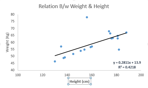
Look at the below example. Here we have identified the best fit line having linear equation y=0.2811x+13.9. Now using this equation, we can find the weight, knowing the height of a person.

Linear_Regression

Linear Regression is of mainly two types: Simple Linear Regression and Multiple Linear Regression. Simple Linear Regression is characterized by one independent variable. And, Multiple Linear Regression(as the name suggests) is characterized by multiple (more than 1) independent variables. While finding best fit line, you can fit a polynomial or curvilinear regression. And these are known as polynomial or curvilinear regression.

Python Code

#Import Library
#Import other necessary libraries like pandas, numpy...
from sklearn import linear_model
#Load Train and Test datasets
#Identify feature and response variable(s) and values must be numeric and numpy arrays
x_train=input_variables_values_training_datasets
y_train=target_variables_values_training_datasets
x_test=input_variables_values_test_datasets
# Create linear regression object
linear = linear_model.LinearRegression()
# Train the model using the training sets and check score
linear.fit(x_train, y_train)
linear.score(x_train, y_train)
#Equation coefficient and Intercept
print('Coefficient: \n', linear.coef_)
print('Intercept: \n', linear.intercept_)
#Predict Output
predicted= linear.predict(x_test)

R Code

#Load Train and Test datasets
#Identify feature and response variable(s) and values must be numeric and numpy arrays
x_train # Train the model using the training sets and check score
linear <- lm(y_train ~ ., data = x)
summary(linear)
#Predict Output
predicted= predict(linear,x_test) 


2. Logistic Regression

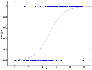
Don’t get confused by its name! It is a classification not a regression algorithm. It is used to estimate discrete values ( Binary values like 0/1, yes/no, true/false ) based on given set of independent variable(s). In simple words, it predicts the probability of occurrence of an event by fitting data to a logit function. Hence, it is also known as logit regression. Since, it predicts the probability, its output values lies between 0 and 1 (as expected).

Again, let us try and understand this through a simple example.

Let’s say your friend gives you a puzzle to solve. There are only 2 outcome scenarios – either you solve it or you don’t. Now imagine, that you are being given wide range of puzzles / quizzes in an attempt to understand which subjects you are good at. The outcome to this study would be something like this – if you are given a trignometry based tenth grade problem, you are 70% likely to solve it. On the other hand, if it is grade fifth history question, the probability of getting an answer is only 30%. This is what Logistic Regression provides you.

Coming to the math, the log odds of the outcome is modeled as a linear combination of the predictor variables.

odds= p/ (1-p) = probability of event occurrence / probability of not event occurrence
ln(odds) = ln(p/(1-p))
logit(p) = ln(p/(1-p)) = b0+b1X1+b2X2+b3X3....+bkXk

Above, p is the probability of presence of the characteristic of interest. It chooses parameters that maximize the likelihood of observing the sample values rather than that minimize the sum of squared errors (like in ordinary regression).

Now, you may ask, why take a log? For the sake of simplicity, let’s just say that this is one of the best mathematical way to replicate a step function. I can go in more details, but that will beat the purpose of this article.

Logistic_RegressionPython Code

#Import Library
from sklearn.linear_model import LogisticRegression
#Assumed you have, X (predictor) and Y (target) for training data set and x_test(predictor) of test_dataset
# Create logistic regression object
model = LogisticRegression()
# Train the model using the training sets and check score
model.fit(X, y)
model.score(X, y)
#Equation coefficient and Intercept
print('Coefficient: \n', model.coef_)
print('Intercept: \n', model.intercept_)
#Predict Output
predicted= model.predict(x_test)

R Code

x # Train the model using the training sets and check score
logistic <- glm(y_train ~ ., data = x,family='binomial')
summary(logistic)
#Predict Output
predicted= predict(logistic,x_test)


Furthermore..

There are many different steps that could be tried in order to improve the model:


3. Decision Tree

This is one of my favorite algorithm and I use it quite frequently. It is a type of supervised learning algorithm that is mostly used for classification problems. Surprisingly, it works for both categorical and continuous dependent variables. In this algorithm, we split the population into two or more homogeneous sets. This is done based on most significant attributes/ independent variables to make as distinct groups as possible. For more details, you can read: Decision Tree Simplified.

IkBzK

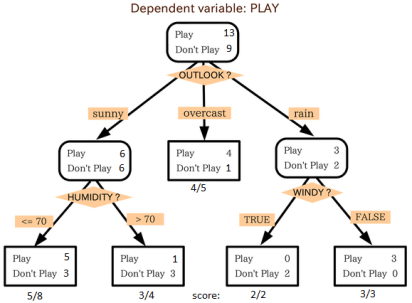
source: statsexchange

In the image above, you can see that population is classified into four different groups based on multiple attributes to identify ‘if they will play or not’. To split the population into different heterogeneous groups, it uses various techniques like Gini, Information Gain, Chi-square, entropy.

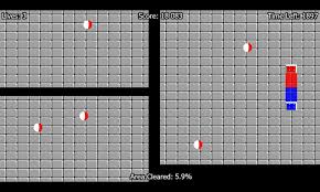
The best way to understand how decision tree works, is to play Jezzball – a classic game from Microsoft (image below). Essentially, you have a room with moving walls and you need to create walls such that maximum area gets cleared off with out the balls.

download

So, every time you split the room with a wall, you are trying to create 2 different populations with in the same room. Decision trees work in very similar fashion by dividing a population in as different groups as possible.

MoreSimplified Version of Decision Tree Algorithms

Python Code

#Import Library
#Import other necessary libraries like pandas, numpy...
from sklearn import tree
#Assumed you have, X (predictor) and Y (target) for training data set and x_test(predictor) of test_dataset
# Create tree object 
model = tree.DecisionTreeClassifier(criterion='gini') # for classification, here you can change the algorithm as gini or entropy (information gain) by default it is gini  
# model = tree.DecisionTreeRegressor() for regression
# Train the model using the training sets and check score
model.fit(X, y)
model.score(X, y)
#Predict Output
predicted= model.predict(x_test)

R Code

library(rpart)
x # grow tree 
fit y_train ~ ., data = x,method="class")
summary(fit)
#Predict Output 
predicted= predict(fit,x_test)


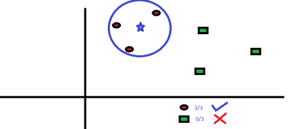
4. SVM (Support Vector Machine)

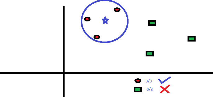
It is a classification method. In this algorithm, we plot each data item as a point in n-dimensional space (where n is number of features you have) with the value of each feature being the value of a particular coordinate.

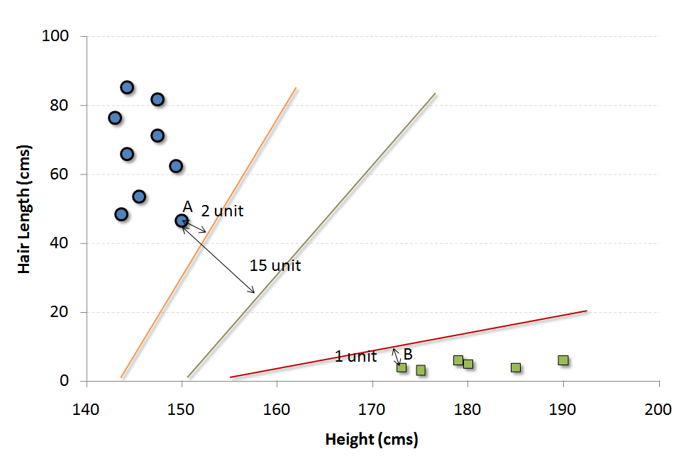
For example, if we only had two features like Height and Hair length of an individual, we’d first plot these two variables in two dimensional space where each point has two co-ordinates (these co-ordinates are known as Support Vectors)

SVM1

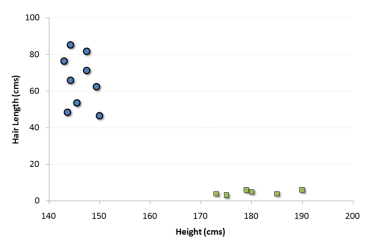
Now, we will find some line that splits the data between the two differently classified groups of data. This will be the line such that the distances from the closest point in each of the two groups will be farthest away.

SVM2

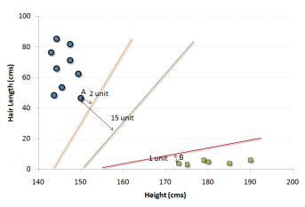
In the example shown above, the line which splits the data into two differently classified groups is the black line, since the two closest points are the farthest apart from the line. This line is our classifier. Then, depending on where the testing data lands on either side of the line, that’s what class we can classify the new data as.

More: Simplified Version of Support Vector Machine

Think of this algorithm as playing JezzBall in n-dimensional space. The tweaks in the game are:

  • You can draw lines / planes at any angles (rather than just horizontal or vertical as in classic game)
  • The objective of the game is to segregate balls of different colors in different rooms.
  • And the balls are not moving.


Python Code

#Import Library
from sklearn import svm
#Assumed you have, X (predictor) and Y (target) for training data set and x_test(predictor) of test_dataset
# Create SVM classification object 
model = svm.svc() # there is various option associated with it, this is simple for classification. You can refer link, for mo# re detail.
# Train the model using the training sets and check score
model.fit(X, y)
model.score(X, y)
#Predict Output
predicted= model.predict(x_test)

R Code

library(e1071)
x # Fitting model
fit <-svm(y_train ~ ., data = x)
summary(fit)
#Predict Output 
predicted= predict(fit,x_test)


5. Naive Bayes

It is a classification technique based on Bayes’ theorem with an assumption of independence between predictors. In simple terms, a Naive Bayes classifier assumes that the presence of a particular feature in a class is unrelated to the presence of any other feature. For example, a fruit may be considered to be an apple if it is red, round, and about 3 inches in diameter. Even if these features depend on each other or upon the existence of the other features, a naive Bayes classifier would consider all of these properties to independently contribute to the probability that this fruit is an apple.

Naive Bayesian model is easy to build and particularly useful for very large data sets. Along with simplicity, Naive Bayes is known to outperform even highly sophisticated classification methods.

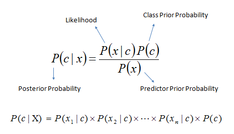
Bayes theorem provides a way of calculating posterior probability P(c|x) from P(c), P(x) and P(x|c). Look at the equation below:
Bayes_rule

Here,

  • P(c|x) is the posterior probability of class (target) given predictor (attribute).
  • P(c) is the prior probability of class.
  • P(x|c) is the likelihood which is the probability of predictor given class.
  • P(x) is the prior probability of predictor.

Example: Let’s understand it using an example. Below I have a training data set of weather and corresponding target variable ‘Play’. Now, we need to classify whether players will play or not based on weather condition. Let’s follow the below steps to perform it.

Step 1: Convert the data set to frequency table

Step 2: Create Likelihood table by finding the probabilities like Overcast probability = 0.29 and probability of playing is 0.64.

Bayes_4

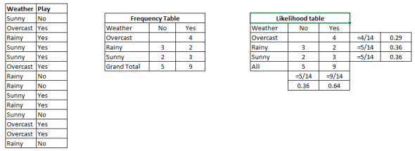
Step 3: Now, use Naive Bayesian equation to calculate the posterior probability for each class. The class with the highest posterior probability is the outcome of prediction.

Problem: Players will pay if weather is sunny, is this statement is correct?

We can solve it using above discussed method, so P(Yes | Sunny) = P( Sunny | Yes) * P(Yes) / P (Sunny)

Here we have P (Sunny |Yes) = 3/9 = 0.33, P(Sunny) = 5/14 = 0.36, P( Yes)= 9/14 = 0.64

Now, P (Yes | Sunny) = 0.33 * 0.64 / 0.36 = 0.60, which has higher probability.

Naive Bayes uses a similar method to predict the probability of different class based on various attributes. This algorithm is mostly used in text classification and with problems having multiple classes.

Python Code

#Import Library
from sklearn.naive_bayes import GaussianNB
#Assumed you have, X (predictor) and Y (target) for training data set and x_test(predictor) of test_dataset
# Create SVM classification object model = GaussianNB() # there is other distribution for multinomial classes like Bernoulli Naive Bayes, Refer link
# Train the model using the training sets and check score
model.fit(X, y)
#Predict Output
predicted= model.predict(x_test)

R Code

library(e1071)
x # Fitting model
fit <-naiveBayes(y_train ~ ., data = x)
summary(fit)
#Predict Output 
predicted= predict(fit,x_test)


6. KNN (K- Nearest Neighbors)

It can be used for both classification and regression problems. However, it is more widely used in classification problems in the industry. K nearest neighbors is a simple algorithm that stores all available cases and classifies new cases by a majority vote of its k neighbors. The case being assigned to the class is most common amongst its K nearest neighbors measured by a distance function.

These distance functions can be Euclidean, Manhattan, Minkowski and Hamming distance. First three functions are used for continuous function and fourth one (Hamming) for categorical variables. If K = 1, then the case is simply assigned to the class of its nearest neighbor. At times, choosing K turns out to be a challenge while performing KNN modeling.

More: Introduction to k-nearest neighbors : Simplified.

KNN

KNN can easily be mapped to our real lives. If you want to learn about a person, of whom you have no information, you might like to find out about his close friends and the circles he moves in and gain access to his/her information!

Things to consider before selecting KNN:

  • KNN is computationally expensive
  • Variables should be normalized else higher range variables can bias it
  • Works on pre-processing stage more before going for KNN like outlier, noise removal

Python Code

#Import Library
from sklearn.neighbors import KNeighborsClassifier
#Assumed you have, X (predictor) and Y (target) for training data set and x_test(predictor) of test_dataset
# Create KNeighbors classifier object model 
KNeighborsClassifier(n_neighbors=6) # default value for n_neighbors is 5
# Train the model using the training sets and check score
model.fit(X, y)
#Predict Output
predicted= model.predict(x_test)

R Code

library(knn)
x # Fitting model
fit <-knn(y_train ~ ., data = x,k=5)
summary(fit)
#Predict Output 
predicted= predict(fit,x_test)


7. K-Means

It is a type of unsupervised algorithm which  solves the clustering problem. Its procedure follows a simple and easy  way to classify a given data set through a certain number of  clusters (assume k clusters). Data points inside a cluster are homogeneous and heterogeneous to peer groups.

Remember figuring out shapes from ink blots? k means is somewhat similar this activity. You look at the shape and spread to decipher how many different clusters / population are present!

splatter_ink_blot_texture_by_maki_tak-d5p6zph

How K-means forms cluster:

  1. K-means picks k number of points for each cluster known as centroids.
  2. Each data point forms a cluster with the closest centroids i.e. k clusters.
  3. Finds the centroid of each cluster based on existing cluster members. Here we have new centroids.
  4. As we have new centroids, repeat step 2 and 3. Find the closest distance for each data point from new centroids and get associated with new k-clusters. Repeat this process until convergence occurs i.e. centroids does not change.

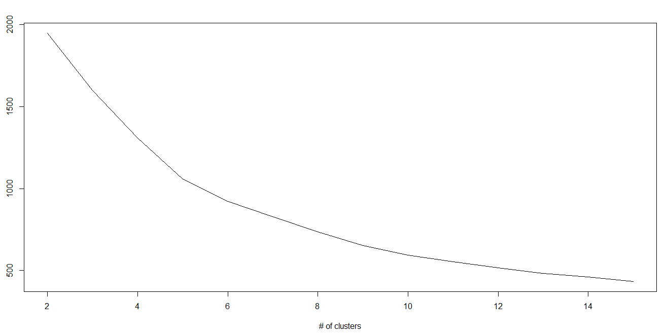
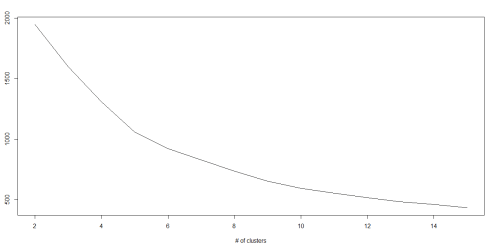
How to determine value of K:

In K-means, we have clusters and each cluster has its own centroid. Sum of square of difference between centroid and the data points within a cluster constitutes within sum of square value for that cluster. Also, when the sum of square values for all the clusters are added, it becomes total within sum of square value for the cluster solution.

We know that as the number of cluster increases, this value keeps on decreasing but if you plot the result you may see that the sum of squared distance decreases sharply up to some value of k, and then much more slowly after that. Here, we can find the optimum number of cluster.

Kmenas

Python Code

#Import Library
from sklearn.cluster import KMeans
#Assumed you have, X (attributes) for training data set and x_test(attributes) of test_dataset
# Create KNeighbors classifier object model 
k_means = KMeans(n_clusters=3, random_state=0)
# Train the model using the training sets and check score
model.fit(X)
#Predict Output
predicted= model.predict(x_test)

R Code

library(cluster)
fit


8. Random Forest

Random Forest is a trademark term for an ensemble of decision trees. In Random Forest, we’ve collection of decision trees (so known as “Forest”). To classify a new object based on attributes, each tree gives a classification and we say the tree “votes” for that class. The forest chooses the classification having the most votes (over all the trees in the forest).

Each tree is planted & grown as follows:

  1. If the number of cases in the training set is N, then sample of N cases is taken at random but with replacement. This sample will be the training set for growing the tree.
  2. If there are M input variables, a number m<
  3. Each tree is grown to the largest extent possible. There is no pruning.

For more details on this algorithm, comparing with decision tree and tuning model parameters, I would suggest you to read these articles:

  1. Introduction to Random forest – Simplified

  2. Comparing a CART model to Random Forest (Part 1)

  3. Comparing a Random Forest to a CART model (Part 2)

  4. Tuning the parameters of your Random Forest model

Python

#Import Library
from sklearn.ensemble import RandomForestClassifier
#Assumed you have, X (predictor) and Y (target) for training data set and x_test(predictor) of test_dataset
# Create Random Forest object
model= RandomForestClassifier()
# Train the model using the training sets and check score
model.fit(X, y)
#Predict Output
predicted= model.predict(x_test)

R Code

library(randomForest)
x # Fitting model
fit summary(fit)
#Predict Output 
predicted= predict(fit,x_test)


9. Dimensionality Reduction Algorithms

In the last 4-5 years, there has been an exponential increase in data capturing at every possible stages. Corporates/ Government Agencies/ Research organisations are not only coming with new sources but also they are capturing data in great detail.

For example: E-commerce companies are capturing more details about customer like their demographics, web crawling history, what they like or dislike, purchase history, feedback and many others to give them personalized attention more than your nearest grocery shopkeeper.

As a data scientist, the data we are offered also consist of many features, this sounds good for building good robust model but there is a challenge. How’d you identify highly significant variable(s) out 1000 or 2000? In such cases, dimensionality reduction algorithm helps us along with various other algorithms like Decision Tree, Random Forest, PCA, Factor Analysis, Identify based on correlation matrix, missing value ratio and others.

To know more about this algorithms, you can read “Beginners Guide To Learn Dimension Reduction Techniques“.

Python  Code

#Import Library
from sklearn import decomposition
#Assumed you have training and test data set as train and test
# Create PCA obeject pca= decomposition.PCA(n_components=k) #default value of k =min(n_sample, n_features)
# For Factor analysis
#fa= decomposition.FactorAnalysis()
# Reduced the dimension of training dataset using PCA
train_reduced = pca.fit_transform(train)
#Reduced the dimension of test dataset
test_reduced = pca.transform(test)
#For more detail on this, please refer  this link.

R Code

library(stats)
pca train, cor = TRUE)
train_reduced  train)
test_reduced  test)


10. Gradient Boosting & AdaBoost

GBM & AdaBoost are boosting algorithms used when we deal with plenty of data to make a prediction with high prediction power. Boosting is an ensemble learning algorithm which combines the prediction of several base estimators in order to improve robustness over a single estimator. It combines multiple weak or average predictors to a build strong predictor. These boosting algorithms always work well in data science competitions like Kaggle, AV Hackathon, CrowdAnalytix.

More: Know about Gradient and AdaBoost in detail

Python Code

#Import Library
from sklearn.ensemble import GradientBoostingClassifier
#Assumed you have, X (predictor) and Y (target) for training data set and x_test(predictor) of test_dataset
# Create Gradient Boosting Classifier object
model= GradientBoostingClassifier(n_estimators=100, learning_rate=1.0, max_depth=1, random_state=0)
# Train the model using the training sets and check score
model.fit(X, y)
#Predict Output
predicted= model.predict(x_test)

R Code

library(caret)
x # Fitting model
fitControl predicted= predict(fit,x_test,type= "prob")[,2] 

GradientBoostingClassifier and Random Forest are two different boosting tree classifier and often people ask about the difference between these two algorithms.

End Notes

By now, I am sure, you would have an idea of commonly used machine learning algorithms. My sole intention behind writing this article and providing the codes in R and Python is to get you started right away. If you are keen to master machine learning, start right away. Take up problems, develop a physical understanding of the process, apply these codes and see the fun!

Did you find this article useful ? Share your views and opinions in the comments section below.

If you like what you just read & want to continue your analytics learning, subscribe to our emailsfollow us on twitter or like our facebook page.

Inside The Mind That Built Google Brain: On Life, Creativity, And Failure

Source: The Huffington Post

(Photo: Jemal Countess/Getty)

Here’s a list of universities with arguably the greatest computer science programs: Carnegie Mellon, MIT, UC Berkeley, and Stanford. These are the same places, respectively, where Andrew Ng received his bachelor’s degree, his master’s, his Ph.D., and has taught for 12 years.

Ng is an icon of the artificial intelligence world with the pedigree to match, and he is not yet 40 years old. In 2011, he founded Google Brain, a deep-learning research project supercharged by Google’s vast stores of computing power and data. Delightfully, one of its most important achievements came when computers analyzing scores of YouTube screenshots were able to recognize a cat. (The New York Timesheadline: “How Many Computers to Identify a Cat? 16,000.”) As Ng explained, “The remarkable thing was that [the system] had discovered the concept of a cat itself. No one had ever told it what a cat is. That was a milestone in machine learning.”

Ng exudes a cheerful but profound calm. He happily discusses the various mistakes and failures of his career, the papers he read but didn’t understand. He wears identical blue oxford shirts each and every day. He is blushing but proud when a colleague mentions his adorable robot-themed engagement photo shoot with his now-wife, a surgical roboticist named Carol Reiley (note his shirt in the photo).

One-on-one, he speaks with a softer voice than anyone you know, though this has not hindered his popularity as a lecturer. In 2011, when he posted videos from his own Stanford machine learning course on the web, over 100,000 people registered. Within a year, Ng had co-founded Coursera, which is today the largest provider of open online courses. Its partners include Princeton and Yale, top schools in China and across Europe. It is a for-profit venture, though all classes are accessible for free. “Charging for content would be a tragedy,” Ng has said.

(Photo: Colson Griffith)

Then, last spring, a shock. Ng announced he was departing Google and stepping away from day-to-day involvement at Coursera. The Chinese tech giant Baidu was establishing an ambitious $300 million research lab devoted to artificial intelligence just down the road from Google’s Silicon Valley headquarters, and Andrew Ng would head it up.

At Baidu, as before, Ng is trying to help computers identify audio and images with incredible accuracy, in realtime. (On Tuesday, Baidu announced it had achieved the world’s best results on a key artificial intelligence benchmark related to image identification, besting Google and Microsoft.) Ng believes speech recognition with 99 percent accuracy will spur revolutionary changes to how humans interact with computers, and how operating systems are designed. Simultaneously, he must help Baidu work well for the millions of search users who are brand new to digital life. “You get queries [in China] that you just wouldn’t get in the United States,” Ng explained. “For example, we get queries like, ‘Hi Baidu, how are you? I ate noodles at a corner store last week and they were delicious. Do you think they’re on sale this weekend?’ That’s the query.” Ng added: “I think we make a good attempt at answering.”

Elon Musk and Stephen Hawking have been sounding alarms over the potential threat to humanity from advanced artificial intelligence. Andrew Ng has not. “I don’t work on preventing AI from turning evil for the same reason that I don’t work on combating overpopulation on the planet Mars,” he has said. AI is many decades away (if not longer) from achieving something akin to consciousness, according to Ng. In the meantime, there’s a far more urgent problem. Computers enhanced by machine learning are eliminating jobs long done by humans. The trend is only accelerating, and Ng frequently calls on policymakers to prepare for the socioeconomic consequences.

At Baidu’s new lab in Sunnyvale, Calif., we spoke to Andrew Ng for Sophia, a HuffPost project to collect life lessons from fascinating people. He explained why he thinks “follow your passion” is terrible career advice and he shared his strategy for teaching creativity; Ng discussed his failures and his helpful habits, the most influential books he’s read, and his latest thoughts on the frontiers of AI.

You recently said, “I’ve seen people learn to be more creative.” Can you explain?

The question is, how does one create new ideas? Is it those unpredictable lone acts of genius, people like Steve Jobs, who are special in some way? Or is it something that can be taught and that one can be systematic about?

I believe that the ability to innovate and to be creative are teachable processes. There are ways by which people can systematically innovate or systematically become creative. One thing I’ve been doing at Baidu is running a workshop on the strategy of innovation. The idea is that innovation is not these random unpredictable acts of genius, but that instead one can be very systematic in creating things that have never been created before.

In my own life, I found that whenever I wasn’t sure what to do next, I would go and learn a lot, read a lot, talk to experts. I don’t know how the human brain works but it’s almost magical: when you read enough or talk to enough experts, when you have enough inputs, new ideas start appearing. This seems to happen for a lot of people that I know.

When you become sufficiently expert in the state of the art, you stop picking ideas at random. You are thoughtful in how to select ideas, and how to combine ideas. You are thoughtful about when you should be generating many ideas versus pruning down ideas.

Now there is a challenge still — what do you do with the new ideas, how can you be strategic in how to advance the ideas to build useful things? That’s another whole piece.

Can you talk about your information diet, how you approach learning?

I read a lot and I also spend time talking to people a fair amount. I think two of the most efficient ways to learn, to get information, are reading and talking to experts. So I spend quite a bit of time doing both of them. I think I have just shy of a thousand books on my Kindle. And I’ve probably read about two-thirds of them.

At Baidu, we have a reading group where we read about half a book a week. I’m actually part of two reading groups at Baidu, each of which reads about half a book a week. I think I’m the only one who’s in both of those groups [laughter]. And my favorite Saturday afternoon activity is sitting by myself at home reading.


Let me ask about your early influences. Is there something your parents did for you that many parents don’t do that you feel had a lasting impact on your life?

I think when I was about six, my father bought a computer and helped me learn to program. A lot of computer scientists learned to program from an early age, so it’s probably not that unique, but I think I was one of the ones that was fortunate to have had a computer and could learn to start to program from a very young age.

Unlike the stereotypical Asian parents, my parents were very laid back. Whenever I got good grades in school, my parents would make a fuss, and I actually found that slightly embarrassing. So I used to hide them. [Laughter] I didn’t like showing my report card to my parents, not because I was doing badly but because of their reaction.

I was also fortunate to have gotten to live and work in many different places. I was born in the U.K., raised in Hong Kong and Singapore, and came to the U.S. for college. Then for my own studies, I have degrees from Carnegie Mellon, MIT, and Berkeley, and then I was at Stanford.

I was very fortunate to have moved to all these places and gotten to meet some of the top people. I interned at AT&T Bell Labs when it existed, one of the top labs, and then at Microsoft Research. I got to see a huge diversity of points of view.

Is there anything about your education or your early career that you would have done differently? Any lessons you’ve learned that people could benefit from?

I wish we as a society gave better career advice to young adults. I think that “follow your passion” is not good career advice. It’s actually one of the most terrible pieces of career advice we give people.

If you are passionate about driving your car, it doesn’t necessarily mean you should aspire to be a race car driver. In real life, “follow your passion” actually gets amended to, “Follow your passion of all the things that happen to be a major at the university you’re attending.”

But often, you first become good at something, and then you become passionate about it. And I think most people can become good at almost anything.

So when I think about what to do with my own life, what I want to work on, I look at two criteria. The first is whether it’s an opportunity to learn. Does the work on this project allow me to learn new and interesting and useful things? The second is the potential impact. The world has an infinite supply of interesting problems. The world also has an infinite supply of important problems. I would love for people to focus on the latter.

I’ve been fortunate to have repeatedly been able to find opportunities that had a lot of potential for impact and also gave me fantastic opportunities to learn. I think young people optimizing for these two things will often have the best careers.

Our team here has a mission of developing hard AI technologies, advanced AI technologies that let us impact hundreds of millions of users. That’s a mission I’m genuinely excited about.


Do you define importance primarily by the number of people who are impacted?

No, I don’t think the number is the only thing that’s important. Changing hundreds of millions of people’s lives in a significant way, I think that’s the level of impact that we can reasonably aspire to. That is one way of making sure we do work that isn’t just interesting, but that also has an impact.

You’ve talked previously about projects of yours that have failed. How do you respond to failure?

Well, it happens all the time, so it’s a long story. [Laughter] A few years ago, I made a list in Evernote and tried to remember all the projects I had started that didn’t work out, for whatever reason. Sometimes I was lucky and it worked out in a totally unexpected direction, through luck rather than skill.

But I made a list of all the projects I had worked on that didn’t go anywhere, or that didn’t succeed, or that had much less to show for it relative to the effort that we put into it. Then I tried to categorize them in terms of what went wrong and tried to do a pretty rigorous post mortem on them.

So, one of these failures was at Stanford. For a while we were trying to get aircraft to fly in formation to realize fuel savings, inspired by geese flying in a V-shaped formation. The aerodynamics are actually pretty solid. So we spent about a year working on making these aircraft fly autonomously. Then we tried to get the airplanes to fly in formation.

But after a year of work, we realized that there is no way that we could control the aircraft with sufficient accuracy to realize fuel savings. Now, if at the start of the project we had thought through the position requirements, we would have realized that with the small aircraft we were using, there is just no way we could do it. Wind gusts will blow you around far more than the precision needed to fly the aircraft in formation.

So one pattern of mistakes I’ve made in the past, hopefully much less now, is doing projects where you do step one, you do step two, you do step three, and then you realize that step four has been impossible all along. I talk about this specific example in the strategy innovation workshop I talked about. The lesson is to de-risk projects early.

I’ve become much better at identifying risks and assessing them earlier on. Now when I say things like, “We should de-risk a project early,” everyone will nod their head because it’s just so obviously true. But the problem is when you’re actually in this situation and facing a novel project, it’s much harder to apply that to the specific project you are working on.

The reason is these sorts of research projects, they’re a strategic skill. In our educational system we’re pretty good at teaching facts and procedures, like recipes. How do you cook spaghetti bolognese? You follow the recipe. We’re pretty good at teaching facts and recipes.

But innovation or creativity is a strategic skill where every day you wake up and it’s a totally unique context that no one’s ever been in, and you need to make good decisions in your completely unique environment. So as far as I can tell, the only was we know way to teach strategic skills is by example, by seeing tons of examples. The human brain, when you see enough examples, learns to internalize those rules and guidelines for making good strategic decisions.

Very often, what I find is that for people doing research, it takes years to see enough examples and to learn to internalize those guidelines. So what I’ve been experimenting with here is to build a flight simulator for innovation strategy. Instead of having everyone spend five years before you see enough examples, to deliver many examples in a much more compressed time frame.

Just as in a flight simulator, if you want to learn to fly a 747, you need to fly for years, maybe decades, before you see any emergencies. But in a flight simulator, we can show you tons of emergencies in a very compressed period of time and allow you to learn much faster. Those are the sorts of things we’ve been experimenting with.

When this lab first opened, you noted that for much of your career you hadn’t seen the importance of team culture, but that you had come to realize its value. Several months in, is there anything you’ve learned about establishing the right culture?

A lot of organizations have cultural documents like, “We empower each other,” or whatever. When you say it, everyone nods their heads, because who wouldn’t want to empower your teammates. But when they go back to their desks five minutes later, do they actually do it? It’s difficult for people to bridge the abstract and the concrete.

At Baidu, we did one thing for the culture that I think is rare. I don’t know of any organization that has done this. We created a quiz that describes to employees specific scenarios — it says, “You’re in this situation and this happens. What do you do: A, B, C, or D?”

No one has ever gotten full marks on this quiz the first time out. I think the quiz interactivity, asking team members to apply specifics to hypothetical scenarios, has been our way of trying to connect the abstract culture with the concrete; what do you actually do when a teammate comes to you and does this thing?

What are some books that had a substantial impact on your intellectual development?

Recently I’ve been thinking about the set of books I’d recommend to someone wanting to do something innovative, to create something new.

The first is “Zero to One“ by Peter Thiel, a very good book that gives an overview of entrepreneurship and innovation.

We often break down entrepreneurship into B2B (“business to business,” i.e., businesses whose customers are other businesses) and B2C (“business to consumer”). For B2B, I recommend “Crossing the Chasm.” For B2C, one of my favorite books is “The Lean Startup,” which takes a narrower view but it gives one specific tactic for innovating quickly. It’s a little narrow but it’s very good in the area that it covers.

Then to break B2C down even further, two of my favorites are “Talking to Humans,” which is a very short book that teaches you how to develop empathy for users you want to serve by talking to them. Also, “Rocket Surgery Made Easy.” If you want to build products that are important, that users care about, this teaches you different tactics for learning about users, either through user studies or by interviews.

Then finally there is “The Hard Thing about Hard Things.“ It’s a bit dark but it does cover a lot of useful territory on what building an organization is like.

For people who are trying to figure out career decisions, there’s a very interesting one: “So Good They Can’t Ignore You.” That gives a valuable perspective on how to select a path for one’s career.

Do you have any helpful habits or routines?

I wear blue shirts every day, I don’t know if you know that. [laughter] Yes. One of the biggest levers on your own life is your ability to form useful habits.

When I talk to researchers, when I talk to people wanting to engage in entrepreneurship, I tell them that if you read research papers consistently, if you seriously study half a dozen papers a week and you do that for two years, after those two years you will have learned a lot. This is a fantastic investment in your own long term development.

But that sort of investment, if you spend a whole Saturday studying rather than watching TV, there’s no one there to pat you on the back or tell you you did a good job. Chances are what you learned studying all Saturday won’t make you that much better at your job the following Monday. There are very few, almost no short-term rewards for these things. But it’s a fantastic long-term investment. This is really how you become a great researcher, you have to read a lot.

People that count on willpower to do these things, it almost never works because willpower peters out. Instead I think people that are into creating habits — you know, studying every week, working hard every week — those are the most important. Those are the people most likely to succeed.

For myself, one of the habits I have is working out every morning for seven minutes with an app. I find it much easier to do the same thing every morning because it’s one less decision that you have to make. It’s the same reason that my closet is full of blue shirts. I used to have two color shirts actually, blue and magenta. I thought that’s just too many decisions. [Laughter] So now I only wear blue shirts.


You’ve urged policymakers to spend time thinking about a future where computing and robotics have eliminated some substantial portion of the jobs people have now. Do you have any ideas about possible solutions?

It’s a really tough question. Computers are good at routine repetitive tasks. Thus far, the main things that computers have been good at automating are tasks where you kind of do the same thing day after day.

Now this can be at multiple points on the spectrum. Humans work on an assembly line, making the same motion for months on end, and now robots are doing some of that work. A midrange challenge might be truck-driving. Truck drivers do very similar things day after day, so computers are trying to do that too. It’s harder than most people think, but automated driving might happen in the next decade or so, we don’t know. Then, even higher-end things, like some radiologists read the same types of x-rays over and over each day. Again, computers may have traction in those areas.

But for the social tasks which are non-routine and non-repetitive, those are the tasks that humans will be better at than computers for quite a period of time, I think. In many of our jobs we do different things every day. We meet different people, we have to arrange different things, solve problems differently. Those things are relatively difficult for computers to do, for now.

The challenge that faces us is that, when the U.S. transformed from an agricultural to a manufacturing and services economy, we had people move from one routine task, such as farming, to a different routine task, such as manufacturing or working call service centers. A large fraction of the population has made that transition, so they’ve been okay, they’ve found other jobs. But many of their jobs are still routine and repetitive.

The challenge that faces us is to find a way to scalably teach people to do non-routine non-repetitive work. Our education system, historically, has not been good at doing that at scale. The top universities are good at doing that for a relatively modest fraction of the population. But a lot of our population ends up doing work that is important but also routine and repetitive. That’s a challenge that faces our educational system.

I think it can be solved. That’s one of the reasons why I’ve been thinking about teaching innovation strategy, teaching creativity strategy. We need to enable a lot of people to do non-routine, non-repetitive tasks. These tactics for teaching innovation and creativity, these flight simulators for innovation, could be one way to get there. I don’t think we’ve figured out yet how to do it, but I’m optimistic it can be done.

You’ve said, “Engineers in China work much harder than the average Silicon Valley engineer. Engineers in Silicon Valley at startups work really hard. At mature companies, I don’t see the same intensity as you do in startups and at Baidu.” Why do you think that is?

I don’t know. I think the individual engineers in China are great. The individual engineers in Silicon Valley are great. The difference I think is the company. The teams of engineers at Baidu tend to be incredibly nimble.

There is much less appreciation for the status quo in the Chinese internet economy and I think there’s a much bigger sense that all assumptions can be challenged and everything is up for grabs. The Chinese internet ecosystem is very dynamic. Everyone sees huge opportunity, everyone sees massive competition. Stuff changes all the time. New inventions arise, and large companies will one day suddenly jump into a totally new business sector.

To give you an idea, here in the United States, if Facebook were to start a brand new web search engine, that might feel like a slightly strange thing to do. Why would Facebook build a search engine? It’s really difficult. But that sort of thing is much more thinkable in China, where there is more of an assumption that there will be new creative business models.


This seems to suggests a different management culture, where you can make important decisions quickly and have them be intelligent and efficient and not chaotic. Is Baidu operating in a unique way that you feel is particularly helpful to its growth?

Gosh, that’s a good question. I’m trying to think what to point to. I think decision making is pushed very far down in the organization at Baidu. People have a lot of autonomy, and they are very strategic. One of the things I really appreciate about the company, especially the executives, is there’s a very clear-eyed view of the world and of the competition.

When executives meet, and the way we speak with the whole company, there is a refreshing absence of bravado. The statements that are made internally — they say, “We did a great job on that. We’re not so happy with those things. This is going well. This is not going well. These are the things we think we should emphasize. And let’s do a post-mortem on the mistakes we made.” There’s just a remarkable lack of bravado, and I think this gives the organization great context on the areas to innovate and focus on.

You’re very focused on speech recognition, among other problems. What are the challenges you’re facing that, when solved, will lead to a significant jump in the accuracy of speech recognition technology?

We’re building machine learning systems for speech recognition. Some of the machine learning technologies we’re using now have been around for decades. It was only in the last several years that they’ve really taken off.

Why is that? I often make an analogy to building a rocket ship. A rocket ship is a giant engine together with a ton of fuel. Both need to be really big. If you have a lot of fuel and a tiny engine, you won’t get off the ground. If you have a huge engine and a tiny amount of fuel, you can lift up, but you probably won’t make it to orbit. So you need a big engine and a lot of fuel.

The reason that machine learning is really taking off now is that we finally have the tools to build the big rocket engine — that is giant computers, that’s our rocket engine. And the fuel is the data. We finally are getting the data that we need.

The digitization of society creates a lot of data and we’ve been creating data for a long time now. But it was just in the last several years we’ve been finally able to build big enough rocket engines to absorb the fuel. So part of our approach, not the whole thing, but a lot of our approach to speech recognition is finding ways to build bigger engines and get more rocket fuel.

For example, here is one thing we did, a little technical. Where do you get a lot of data for speech recognition? One of the things we did was we would take audio data. Other groups use maybe a couple thousand hours of data. We use a hundred thousand hours of data. That is much more rocket fuel than what you see in academic literature.

Then one of the things we did was, if we have an audio clip of you saying something, we would take that audio clip of you and add background noise to it, like a clip recorded in a cafe. So we synthesize an audio clip of what you would sound like if you were speaking in a cafe. By synthesizing your voice against lots of backgrounds, we just multiply the amount of data that we have. We use tactics like that to create more data to feed to our machines, to feed to our rocket engines.

One thing about speech recognition: most people don’t understand the difference between 95 and 99 percent accurate. Ninety-five percent means you get one-in-20 words wrong. That’s just annoying, it’s painful to go back and correct it on your cell phone.

Ninety-nine percent is game changing. If there’s 99 percent, it becomes reliable. It just works and you use it all the time. So this is not just a four percent incremental improvement, this is the difference between people rarely using it and people using it all the time.

So what is the hurdle to 99 percent at this point?

We need even bigger rocket engines and we still need even more rocket fuel. Both are still constrained and the two have to grow together. We’re still working on pushing that boundary.